In teaching some students about survival analysis methods this week, I wanted to demonstrate why we need to use statistical methods that properly allow for right censoring. This post is a brief introduction, via a simulation in R, to why such methods are needed.
To do this, we will simulate a dataset first in which there is no censoring. We first define a variable n for the sample size, and then a vector of true event times from an exponential distribution with rate 0.1:
n <- 10000
set.seed(123)
eventTime <- rexp(n,0.1)
At the moment, we observe the event time for all 10,000 individuals in our study, and so we have fully observed data (no censoring). Because the exponentially distributed times are skewed (you can check with a histogram), one way we might measure the centre of the distribution is by calculating their median, using R’s quantile function:
quantile(eventTime, 0.5)

     50%
6.985061
Since we are simulating the data from an exponential distribution, we can calculate the true median event time, using the fact that the exponential’s survival function is  . If we set
  and solve the equation for
  , we obtain
  for the median survival time. With our value of
  this gives us
-log(0.5)/0.1

6.931472
Our sample median is quite close to the true (population) median, since our sample size is large.
Adding in censoring
Now let’s introduce some censoring. Let’s suppose our study recruited these 10,000 individuals uniformly during the year 2017. To simulate this, we generate a new variable recruitDate as follows:
recruitDate <- 2017+runif(n)We can then plot a histogram to check the distribution of the simulated recruitment calendar times:
hist(recruitDate)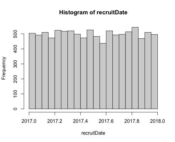
Next we add the individuals’ recruitment date to their eventTime to generate the date that their event takes place:
eventDate <- recruitDate + eventTimeNow let’s suppose that we decide to stop the study at the end of 2019/start of 2020. In this case for those individuals whose eventDate is less than 2020, we get to observe their event time. But for those with an eventDate greater than 2020, their time is censored. We therefore generate an event indicator variable dead which is 1 if eventDate is less than 2020:
dead <- 1*(eventDate<2020)We can now construct the observed time variable. For those with dead==1, this is their eventTime. For those with dead==0, this is the time at which they were censored, which is the difference between their recruitDate and 2020. We thus generate a new variable t as:
t <- eventTime
t[dead==0] <- 2020-recruitDate[dead==0]
Now let’s take a look at the variables we’ve created, with:
> head(cbind(recruitDate,eventTime,dead,t))

     recruitDate  eventTime dead          t
[1,]    2017.961  8.4345726     0 2.0390342
[2,]    2017.277  5.7661027     0 2.7230049
[3,]    2017.702 13.2905487     0 2.2977629
[4,]    2017.959  0.3157736     1 0.3157736

[5,]    2017.705  0.5621098     1 0.5621098
[6,]    2017.797  3.1650122     0 2.2026474
The data we would observe in practice would be each person’s recruitDate, their value of the event indicator dead, and the observed time t. As the above shows, for those individuals with dead==1, the value of t is their eventTime. For those with dead==0, t is equal to the time between their recruitment and the date the study stopped, at the start of 2020.
Next, let’s consider some simple but naive ways of handling the right censoring in the data when trying to estimate the median survival time.
Ignoring the event indicator
One simple approach would be to ignore the censoring completely, in the sense of ignoring the event indicator variable dead. Thus we might calculate the median of the observed time t, completely disregarding whether or not t is an event time or a censoring time:
quantile(t, 0.5)

50%
2.365727
Our estimated median is far lower than the estimated median based on eventTime before we introduced censoring, and below the true value we derived based on the exponential distribution. This happens because we are treating the censored times as if they are event times. For those individuals censored, the censoring times are all lower than their actual event times, some by quite some margin, and so we get a median which is far too small.
Ignoring the censored observations
An arguably somewhat less naive approach would be to calculate the median based only on those individuals who are not censored. If we view censoring as a type of missing data, this corresponds to a complete case analysis or listwise deletion, because we are calculating our estimate using only those individuals with complete data:
quantile(t[dead==1], 0.5)

50%

1.178013
Now we obtain an estimate for the median that is even smaller – again we have substantial downward bias relative to the true value and the value estimated before censoring was introduced. The reason for this large downward bias is that the reason individuals are being excluded from this analysis is precisely because their event times are large. We are estimating the median based on a sub-sample defined by the fact that they had the event quickly. As such, we shouldn’t be surprised that we get a substantially biased (downwards) estimate for the median.
Properly accounting for censoring
To properly allow for right censoring we should use the observed data from all individuals, using statistical methods that correctly incorporate the partial information that right-censored observations provide – namely that for these individuals all we know is that their event time is some value greater than their observed time. We can do this in R using the survival library and survfit function, which calculates the Kaplan-Meier estimator of the survival function, accounting for right censoring:
library(survival)
km <- survfit(Surv(t,dead)~1)
km

Call: survfit(formula = Surv(t, delta) ~ 1)

      n  events  median 0.95LCL 0.95UCL

  10000    2199      NA      NA      NA
This output shows that 2199 events were observed from the 10,000 individuals, but for the median we are presented with an NA, R’s missing value indicator. Why? Plotting the Kaplan-Meier curve reveals the answer:
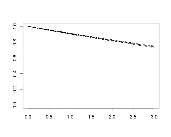
The x-axis is time and the y-axis is the estimate survival probability, which starts at 1 and decreases with time. We see that the x-axis extends to a maximum value of 3. This is because we began recruitment at the start of 2017 and stopped the study (and data collection) at the end of 2019, such that the maximum possible follow-up is 3 years. The curve declines to about 0.74 by three years, but does not reach the 0.5 level corresponding to median survival. This explains the NA for the median – we cannot estimate the median survival time based on these data, at least not without making additional assumptions. The Kapan-Meier estimator is non-parametric – it does not assume a particular distribution for the event times.
If we were to assume the event times are exponentially distributed, which here we know they are because we simulated the data, we could calculate the maximum likelihood estimate of the parameter , and from this estimate the median survival time based on the formula derived earlier. The Kaplan-Meier curve visually makes clear however that this would correspond to extrapolation beyond the range of the data, which we should only data in practice if we are confident in the distributional assumption being correct (at least approximately).
How would you simulate from a Cox proportional hazard model. With and without censoring. I’m looking more from a model validation perspective, where given a fitted cox model, if you are able to simulate back from that model is that simulation representative of the observed data?
Yes you can do this – after fitting the Cox model you have the estimated hazard ratios and you can get an estimate of the baseline hazard function. Together these two allow you to calculate the fitted survival curve for each person given their covariates, and then you can simulate event times for each. To add in censoring you would have to assume some censoring distribution or fit a model for the censoring in the data. For the latter you could fit another Cox model where the ‘events’ are when censoring took place in the original data. I.e. you swap the event indicator values around.
Thanks! Sorry, I missed the reply to the comment earlier.
>another Cox model where the ‘events’ are when censoring took place in the original data
Basically, this would represent a dropout model, for which we need to understand the predictors of the dropout. We can never be sure if the predictors of the dropout model are different than that of the outcome model. I have used this approach before and it seems to work well, but fail when we are unable to capture the predictors of the dropout.
Yes. When you fit a Cox model for the event of interest given some covariates, you are assuming that the censoring time and failure time are conditionally independent given the covariates in your Cox model. You don’t need to actually specify how these covariates influence the hazard for dropout. For a simulation, no doubt there will be other variables which might influence dropout/censoring, but I don’t think you need these to simulate new datasets which (if the two Cox models assumed are correct) will look like the originally observed data.
Nice one, Jonathan! Might also be useful to include a plot with (1) the KM estimator, (2) a naive estimate of the survival curve using just delta=1 people, and (3) a naive survival curve estimate ignoring delta to really drive the point home.
Thanks for the suggestion Lauren! I did this with the second group of students following your suggestion, and will add it to the post!
This introduces censoring in the form of administrative censoring where the necessary assumptions seem very reasonable.
Jonathan, do you ever bother to describe the different types of censoring (type 1, 2 and 3 etc.)? Type 2, if my memory is correct, is fixed pattern censoring where the censoring occurs as soon as some fixed number of failures have occurred. This maintains the the number at risk at the event times, across the alternative data sets required by frequentist methods. If one reads Cox’s original paper, there the likelihood (later called a partial likelihood) is based on the pattern being fixed.
I ask the question as it is possible under Type 2 to define an “exact” CI for the Kaplan Meier estimator equivalent to the Greenford CI.
Thanks James. No I must admit I’ve never gone into the details of the different censoring types much. As I understand it, the random censoring assumption is that each subject’s censoring time is a random variable, independent of their event time. If you recruit randomly over calendar time and then stop the study on a fixed calendar date, then this assumption I think is satisfied.