The t-test is one of the most commonly used tests in statistics. The two-sample t-test allows us to test the null hypothesis that the population means of two groups are equal, based on samples from each of the two groups. In its simplest form, it assumes that in the population, the variable/quantity of interest X follows a normal distribution  in the first group and is
  in the second group. That is, the variance is assumed to be the same in both groups, and the variable is normally distributed around the group mean. The null hypothesis is then that
  .
.
A simple extension allows for the variances to be different in the two groups, i.e. that in the first group, the variable of interest X is distributed  and in the second group as
  . Since often variances can differ between the two groups being tested, it is generally advisable to allow for this possibility.
So, as constructed, the two-sample t-test assumes normality of the variable X in the two groups. On the face of it then, we would worry if, upon inspection of our data, say using histograms, we were to find that our data looked non-normal. In particular, we would worry that the t-test will not perform as it should – i.e. that if the null hypothesis is true, it will falsely reject the null 5% of the time (I’m assuming we are using the usual significance level).
In fact, as the sample size in the two groups gets large, the t-test is valid (i.e. the type 1 error rate is controlled at 5%) even when X doesn’t follow a normal distribution. I think the most direct route to seeing why this is so, is to recall that the t-test is based on the two groups means  and
and  . Because of the central limit theorem, the distribution of these, in repeated sampling, converges to a normal distribution, irrespective of the distribution of X in the population. Also, the estimator that the t-test uses for the standard error of the sample means is consistent irrespective of the distribution of X, and so this too is unaffected by normality. As a consequence, the test statistic continues to follow a
  distribution, under the null hypothesis, when the sample size tends to infinity.
What does this mean in practice? Provided our sample size isn’t too small, we shouldn’t be overly concerned if our data appear to violate the normal assumption. Also, for the same reasons, the 95% confidence interval for the difference in group means will have correct coverage, even when X is not normal (again, when the sample size is sufficiently large). Of course, for small samples, or highly skewed distributions, the above asymptotic result may not give a very good approximation, and so the type 1 error rate may deviate from the nominal 5% level.
Let’s now use R to examine how quickly the sample mean’s distribution (in repeated samples) converges to a normal distribution. We will simulate data from a log-normal distribution – that is, log(X) follows a normal distribution. We can generate random samples from this distribution by exponentiating random draws from a normal distribution. First we will draw a large (n=100000) sample and plots its distribution to see what it looks like:

We can see that its distribution is highly skewed. On the face of it, we would be concerned about using the t-test for such data, which is derived assuming X is normally distributed.
To see what the sampling distribution of looks like, we will choose a sample size n, and repeatedly take draws of size n from the log-normal distribution, calculate the sample mean, and then plot the distribution of these sample means. The following shows a histogram of the sample means for n=3 (from 10,000 repeated samples):
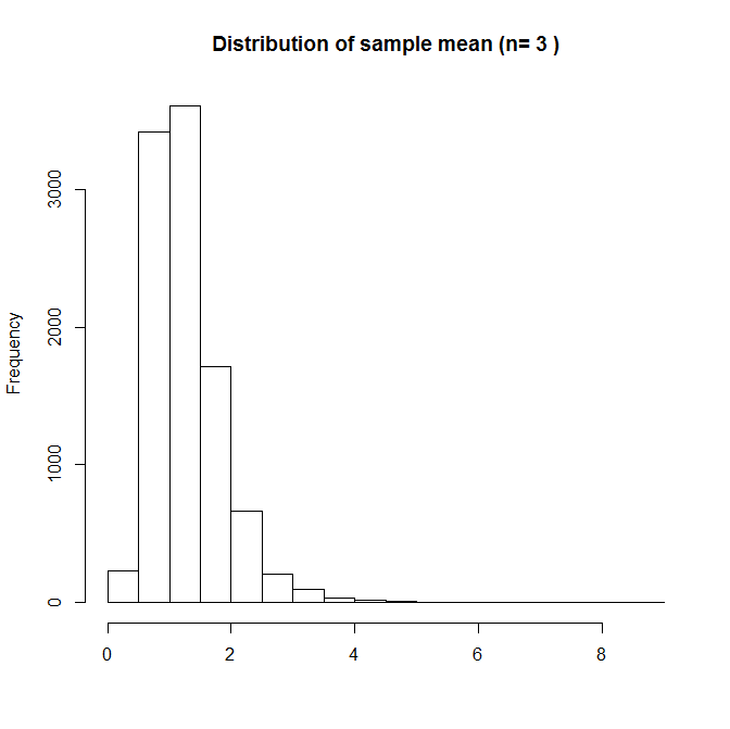
Here the sampling distribution of is skewed. With such a small sample size, if one of the sample has a high value from the tail of the distribution, this will give a sample mean which is quite far from the true mean. If we repeat, but now with n=10:
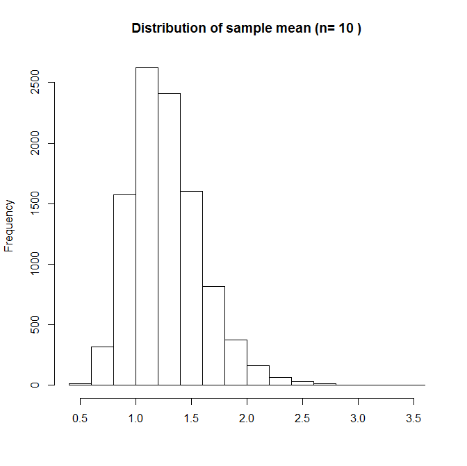
It is now starting to look more normal, but it is still skewed – the sample mean is occasionally large. Notice that x-axis range is now smaller – the variability of the sample mean is now smaller than with n=3. Lastly, we try n=100:
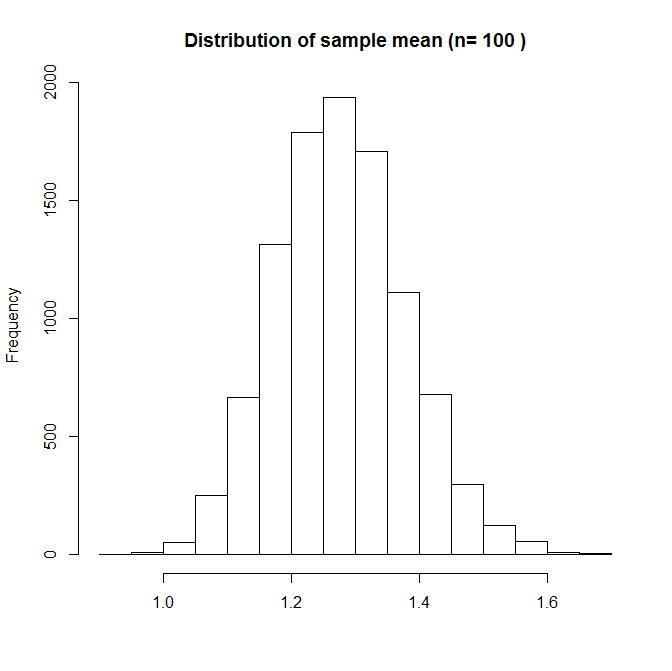
Now the sample mean’s distribution (in repeated samples from the population) looks pretty much normal. When n is large, even though one of our observations might be in the tail of the distribution, all the other observations near the centre of the distribution keep the mean down. This suggests that the t-test should be ok with n=100, for this particular X distribution. A more direct way of checking this would be to perform a simulation study where we empirically estimate the type 1 error rate of the t-test, applied to this distribution with a given choice of n.
Of course if X isn’t normally distributed, even if the type 1 error rate for the t-test assuming normality is close to 5%, the test will not be optimally powerful. That is, there will exist alternative tests of the null hypothesis which have greater power to detect alternative hypotheses.
For more on the large sample properties of hypothesis tests, robustness, and power, I would recommend looking at Chapter 3 of [amazon asin=0387985956&text=’Elements of Large-Sample Theory’] by Lehmann. For more on the specific question of the t-test and robustness to non-normality, I’d recommend looking at this paper by Lumley and colleagues.
Addition – 1st May 2017
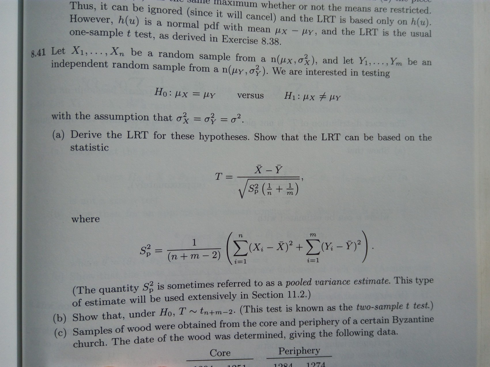
Below Teddy Warner queries in a comment whether the t-test ‘assumes’ normality of the individual observations. The following image is from the book [amazon text=Statistical Inference by Casella and Berger&asin=0534243126], and is provided just to illustrate the point that the t-test is, by its construction, based on assuming normality for the individual (population) values:
This website’s description and explanation of the “normality assumption” of t-tests (and by extension to ANOVA and MANOVA and regression) is simply incorrect. Parametric tests do not assume normality of sample scores nor even of the underlying population of scores from which samples scores are taken. Parametric tests assume that the sampling distribution of the statistic being test is normally distributed – that is, the sampling distribution of the mean or difference in means. Sampling distributions approach normality as sample size increases as shown by the Central Limit Theorem, and the consensus among experts is that with means that are based on sample sizes as small as 30 that the sampling distribution of means is so close to being a normal distribution, that the differences in probabilities in the tails of the normal and almost normal sampling distributions are not worth attention. Also, for any symmetrical distribution of scores, the sampling distribution will be normal.
The normality assumption for Pearson correlation coefficients is also commonly misstated in MANY, if not most, online and textbook sources as requiring the variables being correlated to be normally distributed. X & Y variables do not require normal distributions, but only require that the sampling distribution of r (or t that is used to test the statistical significance of r) be normally distributed. In addition, many sources also misstate the normality assumption for regression and multiple regression as requiring that scores for predictor variables to be normally distributed. Regression only assumes that the residuals of the regression model being fit be normally distributed.
Moreover, the assumption of normality for any statistical test is only relevant if one tests the null hypothesis because the sampling distribution has no effect on the parameter being estimated by the sample – that is, the sample mean and the sample correlation and the sample regression weights are the best unbiased estimates of their corresponding parameters, assuming there are no other “problems” with the data such as outliers, thus not affecting effect size estimates such as the values of r, R-square, b or Cohen’s d. Outliers usually should be trimmed, scores transformed or Winsorized because outliers can distort estimates of any parametric model.
Of course, other assumptions may be important to consider beyond the normality assumption – such as heterscadasticity, independence of observations, and homogeneity of variances. But telling people that their data need to be normally distributed to use t-tests, Pearson correlations, ANOVA, MANOVA, etc. erroneously leads many researchers to use sometimes less powerful non-parametric statistics and thus not to take advantage of more sophisticated parametric models in understanding their data. For example non-parametric models generally cannot deal with interaction effects, but ANOVA, MANOVA and multiple regression can.
Thanks for your comment Teddy. I do believe however that the t-test referred to as the t-test, by its construction, and as I wrote, assumes normality of the underlying observations in the population from which your sample is drawn (see the image I have now included in the bottom of the post, which is from Casella and Berger’s book Statistical Inference). From this it follows that the sampling distribution of the test statistic follows a t-distribution. As you say, and as I wrote and was illustrating, this distribution gets closer and closer to a normal as the sample size increases, as a result of the central limit theorem. This means that provided the sample sizes in the two groups are not too small, the normality assumption of the individual observations is not a concern regarding the test’s size (type 1 error).
You make an interesting point about the assumption being about the distribution of the test statistic, rather than the distribution of the individual observations. I think the point is however that stating that the assumption of a test is regarding the distribution of the test statistic is not easy to exploit. In contrast, assumptions about individual observations (e.g. normality) is something which an analyst can consider and perhaps easily assess from the observed data. In the t-test case, one can examine or consider the plausibility of the observations being normal. But if you tell someone they can only use a test if the test statistic follows a given distribution in repeated samples, how are they do know if and when this will be satisfied?
You wrote “Parametric tests assume that the sampling distribution of the statistic being test is normally distributed” – this of course is not true in general – there are many tests that have sampling distributions other than the normal, for example the F-distribution, or mixtures of chi squared distribution in the case of testing variance components in mixed models.
Teddy is right, here. The t-test doesn’t assume normality. Only in small samples are non-parametric tests necessary. http://www.annualreviews.org/doi/pdf/10.1146/annurev.publhealth.23.100901.140546
y’all are both wrong and the author is right. in support of your criticism you mention the central limit theorem, but the central limit theorem shows that (under certain conditions) sample means converge in distribution to a NORMAL distribution. they do not converge to a T-DISTRIBUTION. the only common situation that will result in a sample mean having a t-distribution is when the population follows a normal distribution. and in that case, it’s not a statement of convergence. the distribution of a sample mean of repeated realizations from a normal distribution IS a t-distribution
The author is right :normality is the condition for which you can have a t-student distribution for the statistic used in the T-test . To have a Student, you must have at least independence between the experimental mean in the numerator and the experimental variance in the denominator, which induces normality. See theorem of Geary.
There is also an another important reason to suppose normality: to have the most powerful test under certain conditions (look to generalization of Pearson theorem).
The author is wrong. The reason this “works” is because as N becomes larger so does the t-stat which means every test you run will be statistically significant. Use the formula provided by the author to confirm this. For large populations, z-score should be used because it doesn’t depend on sample size. In my work, I am using samples of thousands or millions so the t-test becomes irrelevant. Also, if you use z-score to calculate your own confidence interval then you don’t have to worry about the distribution. As long as mean of sample B is greater than 95% of the values of sample A your result is statistically significant.
Can the commenters who claim the author is wrong provide a scientifically robust reference rather than a paper from the field of public health?
According to Montgomery’s “Design and Analysis of Experiments”, the t statistic is defined as the ratio of a z statistic and the square root of a chi-square statistic, the latter divided by the d.f. under the radical. This gives rise to the d.f. for the t statistic. The chi-square is defined as the sum of squared independent z-draws, which are achieved in the t-statistic by dividing the corrected sum of squares of the samples by sigma-squared, the underlying variance of the samples. Hence, the t-statistic assumes the samples are drawn from a normal distribution and may not rely on the central limit theorem to achieve that compliance. That said, the t-test is pretty robust to departures from that assumption.
I am not familiar with the phrasing “a sample mean of repeated realizations from a normal distribution.”
As the distribution of sample means converge to a normal distribution under the CLT as sample size increases, the distribution of the standardized t-score of sample mean (x-bar – mu) / (s/sqrt(n)) converges to a t-distribution. I don’t believe the sample means ever form a t-distribution.