Multiple imputation with splines in R using smcfcs

Tim Morris and I were recently discussing the topic of multiple imputation (MI) of covariates when one wants to assume the covariate affects the outcome via a spline of some kind. We thought that the Substantive Model Compatible Full Conditional Specification (smcfcs) approach to MI should be able to handle this, provided we can specify the spline’s basis functions in a way that smcfcs function (available in R and Stata) can handle. In this post I’ll show that it can be done in R, at least with a simple cubic spline setup.

First, let’s simulate some data where the outcome y depends on a single covariate x via a cubic spline. Before we do that, let’s define a function which returns the positive part of a number or a vector of numbers, which we’ll need for when we define the spline’s basis functions:

#define function that returns positive part
pos <- function(x) {
  res <- x
  res[x<0] <- 0
  res
}

Next we simulate a data of 1,000 individuals using a cubic spline with knots at x=-1,0,1. I simulate the covariate x as being marginally normal:

n <- 1000
set.seed(63412)
x <- 2*rnorm(n)

#define cubic spline basis functions
a <- -1
b <- 0
c <- 1
x1 <- x
x2 <- x^2
x3 <- x^3
#knots at -1, 0, 1
x4 <- pos(x-(-1))^3
x5 <- pos(x-0)^3
x6 <- pos(x-1)^3

#specify true coefficients
beta <- c(0,1,0.1,0.2,-0.1,0.4,0.3)

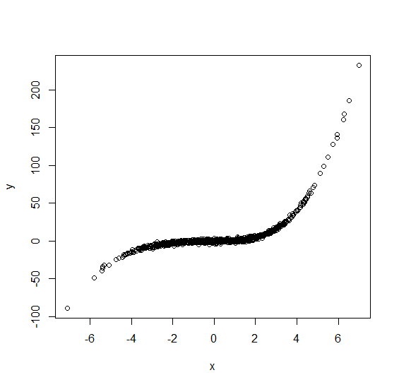
y <- beta[1]+beta[2]*x1+beta[3]*x2+beta[4]*x3+beta[5]*x4+beta[6]*x5+beta[7]*x6+rnorm(n)

Now lets plot this complete data to see what it looks like:

plot(x,y)

Note the residual variation around the conditional mean (regression function) is really small. I’ve done this so that any deficiencies in the imputation process are more obvious. Now we’ll make some x values missing. Here I’ll make them missing completely at random, then put them into a data frame ready for imputation:

#make some x values missing MCAR
x[runif(n)<0.5] <- NA
newdata <- data.frame(x,y)

Let’s now impute the missing values using smcfcs. To do so we’ll need to specify the substantive model, including the spline basis functions as covariates as covariates. To do this we need to remember to use the I() function so that the expressions are evaluated as is:

library(smcfcs)
imps <- smcfcs(newdata, smtype="lm", 
               smformula="y~x+I(x^2)+I(x^3)+I(pos(x-(-1))^3)+I(pos(x-0)^3)+I(pos(x-1)^3)",
               m=1, method=c("norm",""))

Warning message:
In smcfcs.core(originaldata, smtype, smformula, method, predictorMatrix,  :
  Rejection sampling failed 37 times (across all variables, iterations, and imputations). You may want to increase the rejection sampling limit.

I’ve asked for just one imputed dataset. Plotting y vs x in the imputed data we get:

with(imps$impDatasets[[1]], plot(x,y))

This doesn’t look too bad, but comparing to the corresponding plot with complete data, we see larger variation. Moreover, there are a few observations that are a long way from the true conditional mean, which we did not see in the complete data. What’s gone wrong? The answer is the failure in some cases of the rejection sampler, which smcfcs warned us about. For some individuals even after smcfcs’s default 1,000 proposal draws, none were accepted. For these individuals, their imputed x is just a draw from the marginal distribution of x, i.e. imputation not making use of their y value. Let’s re-impute, increasing the rjlimit argument in smcfcs:

#reimpute with larger rjlimit
imps <- smcfcs(newdata, smtype="lm", 
               smformula="y~x+I(x^2)+I(x^3)+I(pos(x-(-1))^3)+I(pos(x-0)^3)+I(pos(x-1)^3)",
               m=1, method=c("norm",""),rjlimit=100000)
Warning message:
In smcfcs.core(originaldata, smtype, smformula, method, predictorMatrix,  :
  Rejection sampling failed 1 times (across all variables, iterations, and imputations). You may want to increase the rejection sampling limit.

with(imps$impDatasets[[1]], plot(x,y))

Now we only get one rejection sampling failure reported, and the plot looks very similar to the one we had with complete data. In most applications we would typically have additional covariates in the substantive model. In this case, the proposal distribution used by smcfcs is based on a model for the partially observed covariate given the other covariates, meaning that failures from rejection sampling are probably lower than in the simple setup used here.

The code used in this post can be downloaded below (you will need to change the file extension from .txt to .R).