Wald vs likelihood ratio test

When taking a course on likelihood based inference, one of the key topics is that of testing and confidence interval construction based on the likelihood function. Usually the Wald, likelihood ratio, and score tests are covered. In this post I’m going to revise the advantages and disadvantages of the Wald and likelihood ratio test. I will focus on confidence intervals rather than tests, because the deficiencies of the Wald approach are more transparently seen here.

Example
As a running example, we’ll use the case of estimating the probability $\pi$ of success in a binomial experiment $Bin(n,\pi)$ . We’ll let X denote the random variable for the number of observed successes, and x its realised value. The likelihood function is simply the binomial probability function, but where the argument is the model parameter $\pi$ . For the binomial distribution the probability mass function is given by

$P(X=x) = \begin{pmatrix}n \\ x \end{pmatrix} \pi^{x} (1-\pi)^{n-x}$

The likelihood function is therefore (with the data x considered fixed)

$L(\pi) = \begin{pmatrix}n \\ x \end{pmatrix} \pi^{x} (1-\pi)^{n-x}$

It is almost always more convenient to work with the log likelihood function, which here is equal to

$l(\pi) = x \log(\pi) +(n-x)\log(1-\pi)$

Here we have ignored the combinatorial term in the likelihood function. We can do this because it only involves n and x, and not the model parameter $\pi$ . This is ok because it turns out that the absolute value of the log likelihood function is not relevant from an inferential perspective, and dropping this term just changes the absolute value of the log likelihood.

To find the maximum likelihood estimate (MLE) of $\pi$ , we first differentiate the log likelihood with respect to it

$l'(\pi) = \frac{x}{\pi} - \frac{n-x}{1-\pi}$

Solving this equation for zero, to find the maximum of the log likelihood, we find

$\hat{\pi} = \frac{x}{n}$

So the MLE is just simply the observed proportion.

The Wald confidence interval
The 95% Wald confidence interval is found as

$\hat{\pi} \pm 1.96 \times SE(\hat{\pi})$

The 1.96 is the 97.5% centile of the standard normal distribution, which is the sampling distribution of the Wald statistic in repeated samples, when the sample size is large.

To find the standard error, we could use the fact that $Var(X)=n\pi(1-\pi)$ for a binomial distribution and derive a standard error estimate from first principles. Instead (we will get the same answer), we will follow the likelihood approach and use the observed (Fisher) information. The information is defined by

$I(\pi) = -\frac{\partial^{2}}{\partial \pi^{2}} l(\pi)$

For the binomial model, we have

$I(\pi) = -\frac{\partial}{\partial \pi} \left\{ \frac{x}{\pi} - \frac{n-x}{1-\pi} \right\} = \frac{x}{\pi^{2}} + \frac{n-x}{(1-\pi)^{2}}$

The standard error is then found as

$SE(\hat{\pi}) = \sqrt{\frac{1}{I(\hat{\pi})}}$

which for the binomial model (with a few lines of algebra) gives

$SE(\hat{\pi}) = \sqrt{\hat{\pi}(1-\hat{\pi})/n}$

Let’s assume n=10 and x=1. Then we have

$SE(\hat{\pi}) = \sqrt{10 \times 0.1 \times 0.9} = 0.0949$

The 95% confidence interval for $\pi$ is then given by

$0.1 \pm 1.96 \times 0.0949$

which gives (-0.086, 0.286). This brings us to the first deficiency of a Wald interval – the interval may include values which are not valid for the parameter in question. Here $\pi$ is a probability, so it makes no sense for the confidence interval to include negative values.

This problem can usually be overcome by calculating the Wald interval on a transformed scale, and then back-transforming the confidence interval limits to the original scale of interest. If we use a transformation which maps the parameter space (in our example the interval (0,1)) to the whole real line, then we are guaranteed to obtain a confidence interval on the original scale which only includes permissible parameter values.

For the binomial probability $\pi$ , this can be achieved by calculating the Wald confidence interval on the log odds scale, and then back-transforming to the probability scale (see Chapter 2.9 of In All Likelihood for the details).

For our n=10 and x=1 example, a 95% confidence interval for the log odds is (-4.263, -0.131). Back transforming to the probability scale, we obtain a 95% confidence interval for $\pi$ of (0.014, 0.467). As desired, this interval only includes valid probabilities, and it is quite different to the Wald interval found on the probability scale. This is a second issue with Wald intervals – they are not transformation invariant. If we calculate our Wald interval on two different scales, and transform back to the probability scale, we will get different confidence intervals.

The Wald based confidence interval has good coverage (i.e. the confidence interval really includes the true value 95% of the time) when the log likelihood function, on the scale on which the Wald interval is constructed, is close to being a quadratic function. The trouble is that while the log likelihood function might be close to quadratic on one scale, as in the log odds for the binomial model, it might not be close to quadratic on another scale, e.g. the probability scale for the binomial model. The following figure shows the log likelihood function (with a constant added so its maximum is zero) plotted against the probability $\pi$ :

Log likelihood function for binomial example with n=10, x=1, plotted against the probability parameter

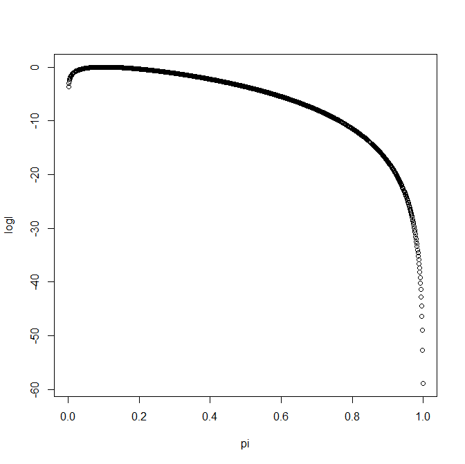
Visually we can see that the log likelihood function, when plotted against $\pi$ is really not quadratic. The following figure shows the same log likelihood function, but now the x-axis is the log odds $\log(\pi/(1-\pi))$ :

Log likelihood function for binomial n=10 x=1 example, against log odds.

Although this is certainly not quadratic, it is much closer to a quadratic than when we plotted against $\pi$ . So we have to be careful to construct the confidence interval on a scale for which the log likelihood is approximately quadratic. For more details on the Wald interval, and a (readable) proof of its validity, I recommend Chapters 2 and 9 of In All Likelihood.

So far things are sounding quite negative for the Wald interval. In reality for many situations Wald intervals are perfectly acceptable, mainly because our statistical software packages calculate the Wald intervals on a scale for which this quadratic approximation of the log likelihood is reasonable. A further advantage is that, in the context of fitting models (e.g. logistic regression), the Wald intervals for each coefficient can be calculated using quantities which are all available from the algorithm used to find the maximum likelihood estimates of the model parameters.

Likelihood ratio confidence interval
The likelihood ratio 95% confidence interval is defined as those values of $\pi$ (or whatever the model parameter is) such that

$2 \log \left\{ \frac{L(\hat{\pi})}{L(\pi)} \right\} \leq 3.84$

The 3.84 is the 95% centile of the chi squared distribution on one degree of freedom (because here we are testing a single parameter), which is the distribution that the likelihood ratio statistic follows (for large sample sizes). For the binomial example where n=10 and x=1, we obtain a 95% CI of (0.006, 0.372). This is still quite different (for the upper limit) from the Wald interval constructed on the log odds scale. This occurs in this example because with such a small sample size the log likelihood is still quite far from a quadratic shape on the log odds scale.

The likelihood (and log likelihood) function is only defined over the parameter space, i.e. over valid values of $\pi$ . Consequently, the likelihood ratio confidence interval will only ever contain valid values of the parameter, in contrast to the Wald interval.

A second advantage of the likelihood ratio interval is that it is transformation invariant. That is, if we find the likelihood ratio confidence interval for the log odds, and then back transform it to the probability scale, we will get an identical confidence interval to the likelihood ratio interval found on the probability scale. This is a consequence of the invariance property of the likelihood function.

When is the likelihood ratio confidence interval valid? It turns out that it will be reasonable when the log likelihood function is approximately quadratic, on some scale. The important point is that we do not need to know what that scale is. In the binomial example, the log likelihood is much closer to quadratic if we consider the log odds. We do not need to know this however – we can find the likelihood ratio interval on the probability scale, without giving any thought as to what scale a quadratic approximation is reasonable. The likelihood ratio interval is therefore valid under a weaker assumption than the Wald interval – that there is some scale (transformation of the model parameter) such that the log likelihood is close to quadratic. In contrast, for the Wald interval to be reasonable we need the log likelihood to be close to quadratic on the scale on which we construct the interval.

For these reasons, the likelihood ratio confidence interval (and corresponding hypothesis test) are preferable statistically to Wald intervals (and tests). However, there are practical disadvantages to the likelihood ratio approach. In the context of regression models, to perform a likelihood ratio test that a particular coefficient is zero we must fit the model which drops the corresponding variable from the model, and compare the maximized likelihood to the likelihood from the original model. We are thus required to fit another model just to perform the test, or construct the confidence interval. If one wanted to write a stats package to fit say a logistic regression and report likelihood ratio intervals for each parameter, in addition to the model of interest, we would have to fit as many models as there are parameters – one for each parameter for which we want to find a likelihood ratio interval.

A second practical disadvantage is that we may not be able to find the likelihood ratio confidence interval limits analytically, and our binomial example is one such situation. By this, I mean you cannot re-arrange the equation to find the lower and upper limits of the interval. Instead, we must resort to using numerical methods like Newton-Raphson to find the limits. For the likelihood ratio interval reported earlier I plotted (using R) the log likelihood ratio statistic against $\pi$ to find the lower and upper limit. Of course this is hardly difficult in the grand scheme of things. However, it is certainly harder than the steps required to find the Wald interval.

In conclusion, although the likelihood ratio approach has clear statistical advantages, computationally the Wald interval/test is far easier. In practice, provided the sample size is not too small, and the Wald intervals are constructed on an appropriate scale, they will usually be reasonable (hence their use in statistical software packages). In small samples however the likelihood ratio approach may be preferred.

Further, a situation in which the Wald approach completely fails while the likelihood ratio approach is still (often) reasonable is when testing whether a parameter lies on the boundary of its parameter space. Situations where this arise include random-effects models, where we are often interested in testing the null hypothesis of whether a random-effects variance parameter is equal to zero.

For further reading on this topic, I suggest a paper by Meeker and Escobar and another by Pawitan, and Pawitan’s book, In All Likelihood.

2 thoughts on “Wald vs likelihood ratio test”

Paul

June 22, 2016 at 3:41 pm

Great article! 🙂

Isn’t the 95% confidence interval for the log odds wrong? I tried to calculate it on my own and I get: (-4.263; -0.131).
Have a nice day!
- Jonathan Bartlett
  
  June 28, 2016 at 6:46 pm
  
  Thanks Paul! You are quite right. The -2.197 I had as the lower limit of the Wald CI for the log odds is actually the MLE of the log odds. I have corrected it – thank you.

2 thoughts on “Wald vs likelihood ratio test”

Leave a ReplyCancel reply