I’ve been teaching a modelling course recently, and have been reading and thinking about the notion of goodness of fit. R squared, the proportion of variation in the outcome Y, explained by the covariates X, is commonly described as a measure of goodness of fit. This of course seems very reasonable, since R squared measures how close the observed Y values are to the predicted (fitted) values from the model.
An important point to remember, however, is that R squared does not give us information about whether our model is correctly specified. That is, it does not tell us whether we have correctly specified how the expectation of the outcome Y depends on the covariate(s). In particular, a high value of R squared does not necessarily mean that our model is correctly specified. This is easiest to illustrate with a simple example.
First we will simulate some data using R. To do this, we randomly generate X values from a standard normal distribution (mean zero, variance one). We then generate the outcome Y equal to X plus a random error, again with a standard normal distribution:
n <- 1000
set.seed(512312)
x <- rnorm(n)
y <- x + rnorm(n)
We can then fit the (correct) linear regression model for Y with X as covariate:
mod1 <- lm(y~x)
summary(mod1)

Call:
lm(formula = y ~ x)

Residuals:
    Min      1Q  Median      3Q     Max
-2.8571 -0.6387 -0.0022  0.6050  3.0716

Coefficients:
            Estimate Std. Error t value Pr(>|t|)
(Intercept)  0.02193    0.03099   0.708    0.479
x            0.93946    0.03127  30.040   <2e-16 ***
---
Signif. codes:  0 ‘***’ 0.001 ‘**’ 0.01 ‘*’ 0.05 ‘.’ 0.1 ‘ ’ 1

Residual standard error: 0.98 on 998 degrees of freedom
Multiple R-squared:  0.4748,    Adjusted R-squared:  0.4743
F-statistic: 902.4 on 1 and 998 DF,  p-value: < 2.2e-16
Since we have specified the model correctly, we are not surprised that the parameter estimates of the intercept and slope are close to the values used to simulate the data (0 for the intercept, 1 for the slope). We also note that the R squared value is 0.47, indicating that X explains an estimated 47% of the variation in Y.
We can also plot the data, overlayed with the fitted line from the model:
plot(x,y)
abline(mod1)
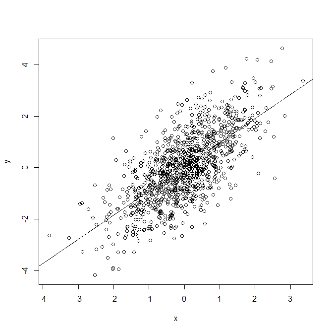
Now let's re-generate the data, but generating Y such that its expectation is an exponential function of X:
n <- 1000
set.seed(512312)
x <- rnorm(n)
y <- exp(x) + rnorm(n)
In practice of course, we don't simulate our data - we observe or collect the data and then try to fit a reasonable model to it. So, as before, we might start by fitting a simple linear regression model, which assumes the expectation of Y is a linear function of X:
mod2 <- lm(y~x)
summary(mod2)

Call:
lm(formula = y ~ x)

Residuals:
    Min      1Q  Median      3Q     Max
-3.5022 -0.9963 -0.1706  0.6980 21.7411

Coefficients:
            Estimate Std. Error t value Pr(>|t|)
(Intercept)  1.65123    0.05220   31.63   <2e-16 ***
x            1.53517    0.05267   29.15   <2e-16 ***
---
Signif. codes:  0 ‘***’ 0.001 ‘**’ 0.01 ‘*’ 0.05 ‘.’ 0.1 ‘ ’ 1

Residual standard error: 1.651 on 998 degrees of freedom
Multiple R-squared:  0.4598,    Adjusted R-squared:  0.4593
F-statistic: 849.5 on 1 and 998 DF,  p-value: < 2.2e-16
Unlike in the first case, the parameter estimates we obtain (1.65, 1.54) are not unbiased estimates of the parameters in the 'true' data generating mechanism, in which the expectation of Y is a linear function of exp(X). Also, we see that we obtain an R squared value of 0.46, indicating again that X (included linearly) explains quite a large amount of the variation in Y. We might take this to mean that the model we have used, that the expectation of Y is linear in X, is reasonable. However, if we again plot the observed data, and overlay it with the fitted line:
 data and overlayed fitted line. The model we have used here is not correctly specified.")
Overlaying the fitted line onto the observed data makes clear that the model we have used is not correctly specified, despite the fact that the R squared value is quite large. In particular we see that for both low and high values of X, the fitted values are too small. This is obviously a consequence of the fact that the expectation of Y depends on exp(X), whereas the model we have used assumes it is a linear function of X.
This simple example illustrates that, although R squared is an important measure, a high value does not mean our model is correctly specified. Arguably a better way of describing R squared is as a measure of 'explained variation'. For assessing whether our model is correctly specified, we should make use of model diagnostic techniques, such as plots of residuals against the covariates or the linear predictor.
Good point here. But I think Pearson’s R-sqaured are defined as to describe the LINEAR relationship between variables. Therefore, it kind makes sense that it does not work well when the relationship is not linear.
Thanks. I’m not sure that’s strictly correct though. The R squared in linear regression represents the proportion of squared variation in the outcome explained by the linear predictor. The linear predictor could allow the mean to depend on higher order functions of covariates. So you could fit a model where the outcome’s mean is assumed to be a linear function of X and X^2, have a high R squared value, but the true mean be some other function of X such that the model is not correctly specified, and does not really ‘fit the data’, and this was the point I was trying to make.
So what your mean is a high value of R squared couldn’t guarantee the right regression model was proposed. So, how could we identify which model is better.For example, during your illustration, the exp() is better?
Understood that a high R-squared doesn’t mean a correctly specified model. Does a low R-squared mean an incorrectly specified model? Why or why not?
No it doesn’t. The model can still be well specified with a low R-squared – low R-squared simply means the predictors don’t explain a large proportion of the variability in the outcome.
Thank´s for the post. What about using R squared as a first approach to compare the goodness of fit of two models. Let´s say, case 1: two nested models, case 2: to models that differ in a transformation of Y.
For 1, yes that’s fine. For case 2, do you mean two models with the same X but different transformations of Y? Comparing R^2 here would be ok here too – you are seeing whether a linear relationship (assuming you have just put X in linearly in the models) between X and transformed Y fits better/worse than for untransformed Y.