From DAGs to potential outcomes via Single World Intervention Graphs

Directed acyclic graphs (DAGs) are an exceptionally useful tool for graphically depicting assumptions about causal structure. An accompanying rich theory has been developed which enables one to (for example) determine if there exist sets of variables which if adjusted for would enable estimation of the causal effect of one (the exposure) of the variables in the DAG on another (the outcome). Personally I have found them very useful for thinking about missing data assumptions (see ‘Understanding missing at random dropout using DAGs‘, for example).

Separately, I have similarly found the concepts of potential outcomes (counterfactuals), as used extensively by Jamie Robins, very useful. The concept of defining causal effects as the difference between what one would observe if an exposure is set to one level as opposed to set to another level is extremely intuitive.

For many years I must admit I did not even notice that there was somewhat of a disconnect between DAGs and potential outcomes, in the sense that if you draw a DAG encoding your causal assumptions about a process in the world, the DAG does not contain any potential outcomes. As I noted earlier, DAGs have rules/conditions about when one can estimate the causal effect of an exposure in the presence of confounding, and the potential outcomes framework similarly has conditions sufficient to estimate the causal effect of exposure. But because the DAG doesn’t contain potential outcomes, it seemed difficult to directly connect these two frameworks. In particular, the no confounding or exchangeability assumption in the potential outcome framework can’t seemingly be checked from a DAG, since the DAG doesn’t contain the potential outcomes.

This post is about Single-World Intervention Graphs, which for me felt like a bit of revelation when I discovered them. They allow one to take a DAG and determine what would happen if one were to intervene to set the value of certain variables to certain values. In doing so, potential outcomes emerge into the graph, and enable us to (for example) check the exchangeability assumption. I draw heavily on Hernán and Robins’ Causal Inference book.

DAG with simple confounding

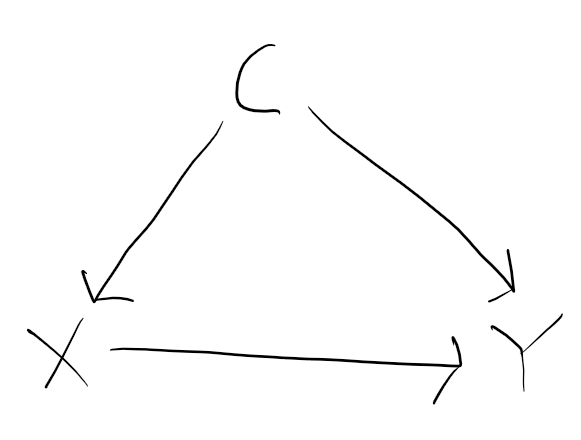
To make clear what I’m talking about, let’s take the simplest possible DAG where we have some confounding. Let’s suppose we have a confounder C, an exposure X, and an outcome Y, with DAG:

Here there is a ‘backdoor’ path from exposure X to outcome Y via the confounder C. It is a ‘backdoor’ path because it is a non-causal path which remains if we delete the causal path from X to Y. Here C satisfies the ‘backdoor criterion’ because all backdoor paths (here there is only one) are blocked if we condition on C. DAG theory then implies we can estimate (identify) the causal effect of X on Y by adjusting for C.

Conditional exchangeability

Let Y(0) and Y(1) denote the potential outcomes for Y if we were to intervene to set exposure X to levels 0 and 1 respectively. More generally, Y(x) denotes the potential outcome if we were to set exposure X to some level x. The conditional exchangeability assumption here states that Y(x) is conditionally independent of X (the exposure level assigned by ‘nature’), conditional on C, for both x=0 and x=1. In words, this means that conditional on C, the assignment of exposure (X) is statistically independent of the potential outcome Y(0), and also statistically independent of the potential outcome Y(1). It doesn’t however seem possible to directly conclude that this assumption holds from the DAG we drew above.

Single-world intervention graph

Single-world intervention graphs (see Richardson and Robins and Hernán and Robins’ Section 7.5) take an assumed DAG for the actual world and show the counterfactual dependencies that would exist if we were to intervene to set the value of one (or more) of the variables to particular values.

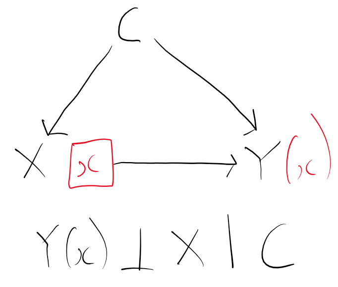
To convert the DAG to a SWIG, we split the exposure (treatment) node we are intervening on into two. The right hand side node becomes x, the value we are intervening to set the exposure to (e.g. 0 or 1). All the arrows that pointed from X in the DAG now point from this new right hand node x in the SWIG. The left hand node X remains, and continues to represent the value exposure would have taken naturally in the real (non intervened world). All arrows in the DAG which originally pointed to X still point to X in the SWIG. Lastly, the variable Y in the DAG becomes the potential outcome Y(x), because X is an ancestor of Y in the original DAG. The resulting SWIG is:

From the SWIG, we can now deduce that Y(x) is independent of X conditional on C, since there are no open paths between Y(x) and X once we condition on C.

I really like the way SWIGs are able to connect the DAG world to the potential outcome framework. For my current work they are proving invaluable in determining independencies between potential outcomes under particular interventions under assumed DAGs which are somewhat more complicated than the one above. For further reading, I highly recommend Richardson and Robins’ ‘Single World Intervention Graphs: A Primer’ paper.