The mean of residuals in linear regression is always zero

In an introductory course on linear regression one learns about various diagnostics which might be used to assess whether the model is correctly specified. One of the assumptions of linear regression is that the errors have mean zero, conditional on the covariates. This implies that the unconditional or marginal mean of the errors have mean zero.

One might be tempted to check whether this latter property is true using the sample data. We can estimate the individual errors by the residuals:

$\begin{eqnarray*}\hat{\epsilon}_{i} = Y_{i} - X^{T}_{i} \hat{\beta}\end{eqnarray*}$

where $Y_{i}$ denotes the outcome/response for unit i, $\hat{\beta}$ represents the ordinary least squares (OLS) estimator, and $X_{i}$ is a column vector of predictors for unit i, for which the first element is 1, corresponding to the intercept.

The OLS estimator is given by $\hat{\beta} = (X^{T} X)^{-1} X^{T} Y$ where $X$ denotes the $n \times p$ matrix of covariate values across the $n$ units and $p$ predictors (including the intercept). Multiplying this equation by $X^{T} X$ and re-arranging we obtain that

$\begin{eqnarray*} X^{T} (Y-X \hat{\beta}) = 0 \end{eqnarray*}$

The first row of $X^{T}$ consists solely of 1s, corresponding to the intercept, and the term in brackets is the vector of residuals, and so this equation implies that

$\begin{eqnarray*} \sum^{n}_{i=1} Y_{i} - X^{T}_{i} \hat{\beta} = 0\end{eqnarray*}$

so that $\sum^{n}_{i=1} \hat{\epsilon}_{i} = 0$ . Thus the sum and mean of the residuals from a linear regression will always equal zero, and there is no point or need in checking this using the particular dataset and $\hat{\beta}$ we obtain.

A simple illustration using R

Let’s illustrate this with a simple simulation in R. First we simulate some data where the outcome $Y$ depends quadratically on a single covariate $X$ :

set.seed(1234)
n <- 100
x <- rnorm(n)
y <- x^2 + rnorm(n)

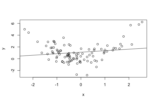
Let’s first plot the simulated data and overlay the OLS line, (wrongly) including $X$ as covariate:

plot(x,y)
abline(lm(y~x))

We can see clearly that the model is not fitting well for low and high values of X, and is not capturing the quadratic association. We now fit this linear model and calculate the mean of the residuals:

mod <- lm(y ~ x)
mean(mod$residuals)
[1] -3.055715e-17

As we expect from the above theory, the overall mean of the residuals is zero. It is not exactly zero because of tiny numerical errors.

Calculating the overall mean of the residuals thus gives us no information about whether we have correctly modelled how the mean of Y depends on X. R’s lm function gives us a variety of diagnostic plots, and these can help us to diagnose misspecification. The first one plots the residuals against the fitted values:

plot(mod,1)

Here with a single covariate X included linearly the fitted values are just a linear combination of X. The red line shows a lowess smoother, and clearly indicates that the mean of the residuals is above zero for low and high fitted values, indicating that we have not correctly modelled how the mean of Y depends on X.

The mean of residuals in linear regression is always zero

A simple illustration using R

You may also be interested in:

Leave a ReplyCancel reply